CS-466/566: Math for AI
Module 01: Probability, Conditional Probability, and Bayes Rule
The University of Alabama
2026-04-08
TABLE OF CONTENTS
The Third Pillar
We have built two pillars of mathematical thinking for AI:
Today’s goal: Build the language and rules of probability, then see how Bayes rule lets AI systems update beliefs from evidence.
Why Does AI Need Probability?
Most AI problems are not deterministic. We deal with:
- Noisy sensors and incomplete information
- Uncertain labels and ambiguous inputs
- Imperfect models and uncertain predictions
Real examples:
- A classifier predicts “cat” with 0.82 confidence
- A medical AI flags disease risk based on symptoms
- A spam filter estimates whether an email is spam
- A robot reasons with noisy camera measurements
Probability is the mathematical language for uncertainty.
TABLE OF CONTENTS
Experiment, Outcome, Sample Space
Experiment is a process with an uncertain result.
Examples: toss a coin, roll a die, test an email for spam
Outcome is one possible result of the experiment.
Examples: Heads, Tails; or 1, 2, 3, 4, 5, 6
Sample Space (\(S\) or \(\Omega\)): The set of all possible outcomes.
\[S_{\text{coin}} = \{H, T\} \qquad S_{\text{die}} = \{1,2,3,4,5,6\}\]
AI example: Testing whether an email is spam → \(S = \{\text{spam}, \text{not-spam}\}\)
Events
An event is a set of outcomes, a subset of the sample space.
Example: Rolling a die. Let \(A\) = “even number”: \[A = \{2, 4, 6\} \subseteq S\]
Example: Let \(B\) = “number greater than 4”: \[B = \{5, 6\} \subseteq S\]
In probability, we assign probabilities to events, not just individual outcomes. This is important because in AI, we often care about compound conditions.
TABLE OF CONTENTS
Probability Axioms
Probability is a function that assigns a number between 0 and 1 to events. It satisfies three axioms:
Interpretation: Probabilities are non-negative, they sum to 1 over the whole space, and disjoint events simply add.
Complement Rule
If \(A^c\) means “not \(A\),” then:
\[P(A^c) = 1 - P(A)\]
Example: If the probability of rain is \(0.3\), then: \[P(\text{no rain}) = 1 - 0.3 = 0.7\]
Intuition: Something either happens or it doesn’t. The probabilities must add to 1.
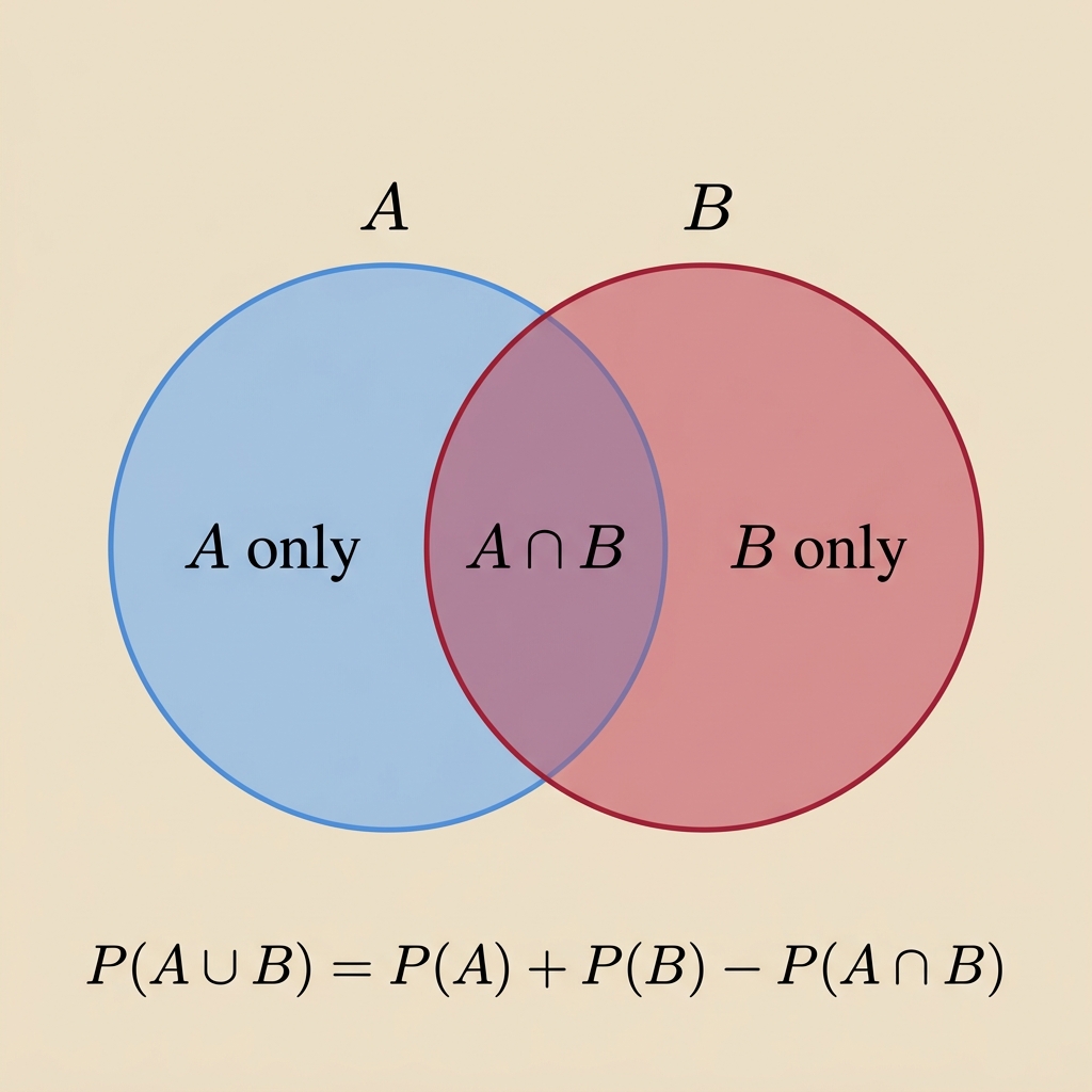
Addition Rule
For any two events \(A\) and \(B\):
\[P(A \cup B) = P(A) + P(B) - P(A \cap B)\]
Why subtract? The overlap \(A \cap B\) gets counted twice; once in \(P(A)\) and once in \(P(B)\).
Example:
- \(P(A)=0.5\), \(P(B)=0.4\), \(P(A \cap B)=0.2\)
- \(P(A \cup B)=0.5+0.4-0.2=0.7\)
Joint and Marginal Probability
Two kinds of probability appear constantly in AI:
Key distinction: Joint probability considers two events together; marginal probability considers one event alone.
TABLE OF CONTENTS
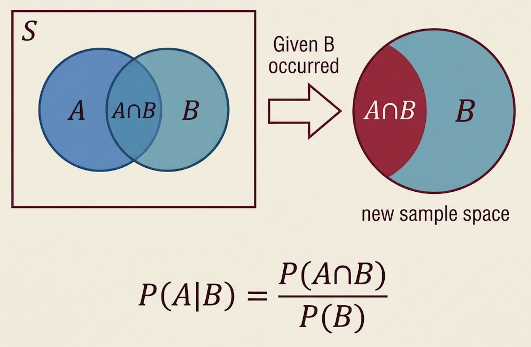
What Is Conditional Probability?
Conditional probability answers:
What is the probability of \(A\) after we already know that \(B\) happened?
\[P(A \mid B) = \frac{P(A \cap B)}{P(B)}, \qquad P(B)>0\]
Intuition: Once we know \(B\) happened, the sample space shrinks to just \(B\). Among those outcomes, how many also satisfy \(A\)?
Example: Drawing a Card
Draw one card from a standard 52-card deck. What is the probability of \(P(A \mid B)\)?
- \(A\): card is a King
- \(B\): card is a face card (J, Q, K)
Since every King is also a face card: \(P(A \cap B) = P(A) = \frac{4}{52}\)
\[P(A \mid B) = \frac{P(A \cap B)}{P(B)} = \frac{4/52}{12/52} = \frac{4}{12} = \frac{1}{3}\]
Interpretation: If you know the card is a face card, the chance it is a King becomes \(1/3\) , up from \(4/52 \approx 7.7\%\) without that knowledge.
A Critical Distinction for AI
Consider a medical test. Let:
- \(D\): patient has the disease
- \(T\): test result is positive
\(P(T \mid D)\)
“How likely is a positive test if the patient is sick?”
This is the test’s sensitivity.
\(P(D \mid T)\)
“How likely is the patient actually sick given a positive test?”
This is the diagnostic question.
⚠️ These are NOT the same! Confusing \(P(A \mid B)\) with \(P(B \mid A)\) is one of the most common errors in probabilistic reasoning.
TABLE OF CONTENTS
Independent Events
Two events \(A\) and \(B\) are independent if knowing one gives no information about the other.
\[P(A \cap B) = P(A) \cdot P(B) \qquad \Longleftrightarrow \qquad P(A \mid B) = P(A)\]
Example: Flipping a fair coin twice.
- \(A\): first toss is Heads, \(P(A) = 1/2\)
- \(B\): second toss is Heads, \(P(B) = 1/2\)
\[P(A \cap B) = \frac{1}{4} = \frac{1}{2} \cdot \frac{1}{2} = P(A) \cdot P(B) \quad \checkmark\]
Interpretation: The outcome of the first flip tells us nothing about the second flip.
This is the core idea behind i.i.d. data in machine learning.
Independence ≠ Mutual Exclusivity
Students often confuse these; they are opposite concepts:
Knowing \(B\) does not change \(P(A)\).
\[P(A \cap B) = P(A) \cdot P(B)\]
Events can happen together.
Events cannot happen together.
\[P(A \cap B) = 0\]
Knowing \(B\) guarantees \(A\) didn’t happen.
⚠️ If events are mutually exclusive and both have nonzero probability, they are NOT independent. Mutual exclusivity means maximum dependence; the events are anti-correlated!
TABLE OF CONTENTS
Deriving Bayes Rule
Start from the definition of conditional probability:
From \(A\) given \(B\): \(\quad P(A \mid B) = \dfrac{P(A \cap B)}{P(B)}\)
From \(B\) given \(A\): \(\quad P(B \mid A) = \dfrac{P(A \cap B)}{P(A)}\)
Both give us \(P(A \cap B)\): \[P(A \cap B) = P(B \mid A) \cdot P(A)\]
Substitute into the first equation:
\[\boxed{P(A \mid B) = \frac{P(B \mid A) \cdot P(A)}{P(B)}}\]
Interpreting Bayes Rule
Bayes rule tells us how to update our beliefs after observing evidence:
\[\underbrace{P(A \mid B)}_{\text{Posterior}} = \frac{\overbrace{P(B \mid A)}^{\text{Likelihood}} \cdot \overbrace{P(A)}^{\text{Prior}}}{\underbrace{P(B)}_{\text{Evidence}}}\]
| Term | Symbol | Meaning |
|---|---|---|
| Prior | \(P(A)\) | What we believed before seeing evidence |
| Likelihood | \(P(B \mid A)\) | How likely the evidence is if \(A\) is true |
| Evidence | \(P(B)\) | Overall probability of observing this evidence |
| Posterior | \(P(A \mid B)\) | Updated belief after seeing evidence |
AI Application: Spam Filtering
The same reasoning powers one of the earliest AI applications:
- \(S\): email is spam
- \(W\): email contains the word “winner”
Then Bayes tells us:
\[P(S \mid W) = \frac{P(W \mid S) \cdot P(S)}{P(W)}\]
| Term | Meaning |
|---|---|
| \(P(S)\) | Prior: Overall fraction of emails that are spam |
| \(P(W \mid S)\) | Likelihood: How often spam emails contain “winner” |
| \(P(W)\) | Evidence: How often any email contains “winner” |
| \(P(S \mid W)\) | Posterior: Updated spam probability after seeing “winner” |
This is exactly how Naive Bayes classifiers work: one of the simplest and most effective ML algorithms.
Multi-word Naive Bayes
If an email contains words \(w_1, w_2, \dots, w_n\), our goal is to find the probability of spam \(S\):
\[P(S \mid w_1, w_2, \dots, w_n)\]
By Bayes rule, we can rewrite this as:
\[P(S \mid w_1, \dots, w_n) = \frac{P(w_1, \dots, w_n \mid S) \, P(S)}{P(w_1, \dots, w_n)}\]
💡 The “Naive” part: It assumes words appear independently from each other: \[P(w_1, \dots, w_n \mid S) = P(w_1 \mid S) \cdot P(w_2 \mid S) \dots P(w_n \mid S)\]
AI Application: Classification
More generally, AI classification can be framed as Bayesian inference:
Given observed features \(X\) and a class label \(C\):
\[P(C \mid X) = \frac{P(X \mid C) \cdot P(C)}{P(X)}\]
In words: To classify a data point, ask:
- How common is this class? → Prior \(P(C)\)
- How well do the features match this class? → Likelihood \(P(X \mid C)\)
- Combine them with Bayes rule → Posterior \(P(C \mid X)\)
Many AI systems, from spam filters to medical diagnosis to autonomous robots, use this probabilistic reasoning at their core.
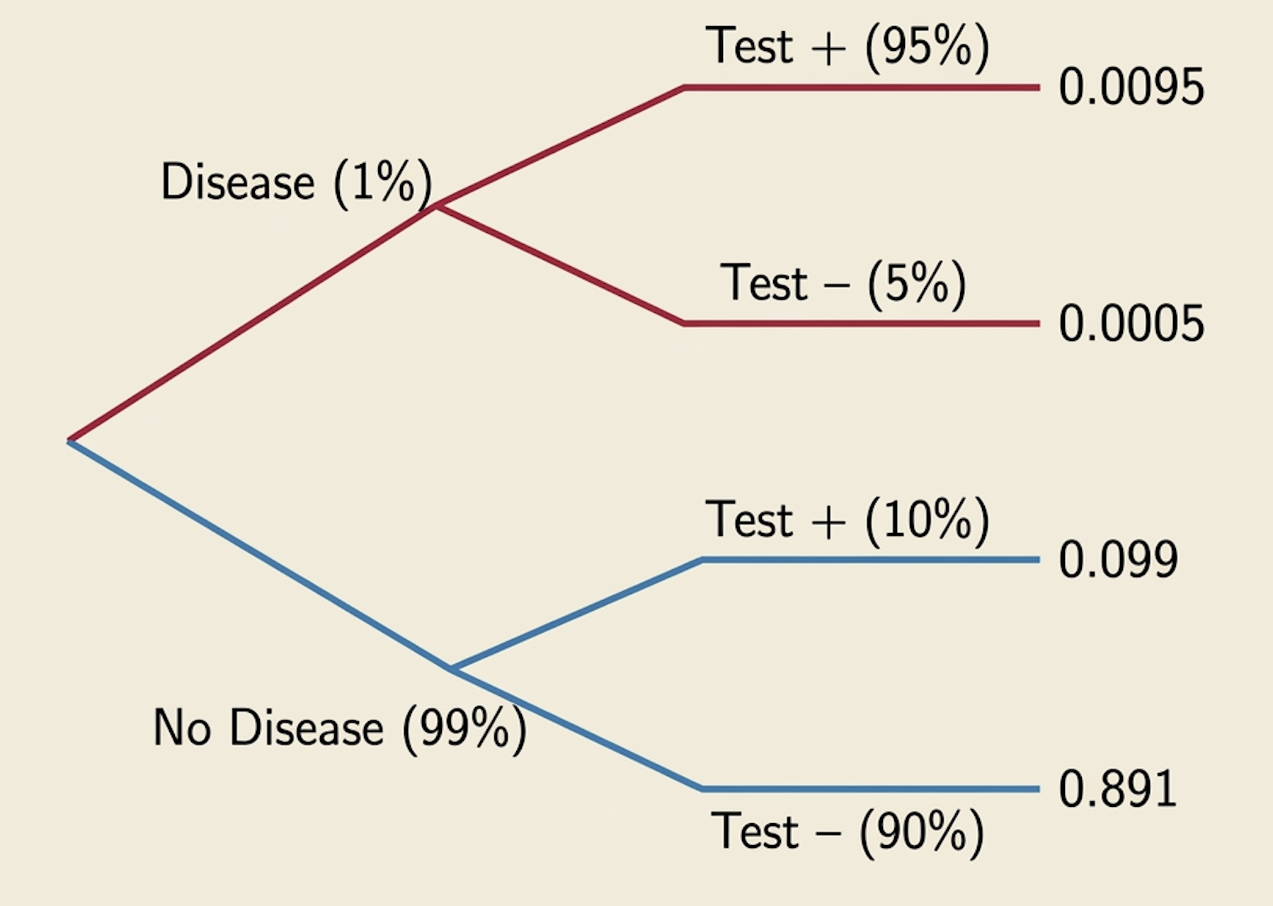
Disease Testing: Setup
Suppose:
- 1% of people have a disease: \(\quad P(D) = 0.01\)
- Test is 95% sensitive: \(\quad P(T^+ \mid D) = 0.95\)
- False positive rate is 10%: \(\quad P(T^+ \mid D^c) = 0.10\)
Question: A person tests positive. What is the probability they actually have the disease?
\[P(D \mid T^+) = \; ?\]
Disease Testing: Computation
Apply Bayes Rule: \(\quad P(D \mid T^+) = \dfrac{P(T^+ \mid D) \cdot P(D)}{P(T^+)}\)
Step 1: Compute \(P(T^+)\) using the Law of Total Probability:
\[P(T^+) = P(T^+ \mid D) \cdot P(D) + P(T^+ \mid D^c) \cdot P(D^c)\] \[= 0.95 \times 0.01 + 0.10 \times 0.99 = 0.0095 + 0.099 = 0.1085\]
Step 2: Apply Bayes Rule:
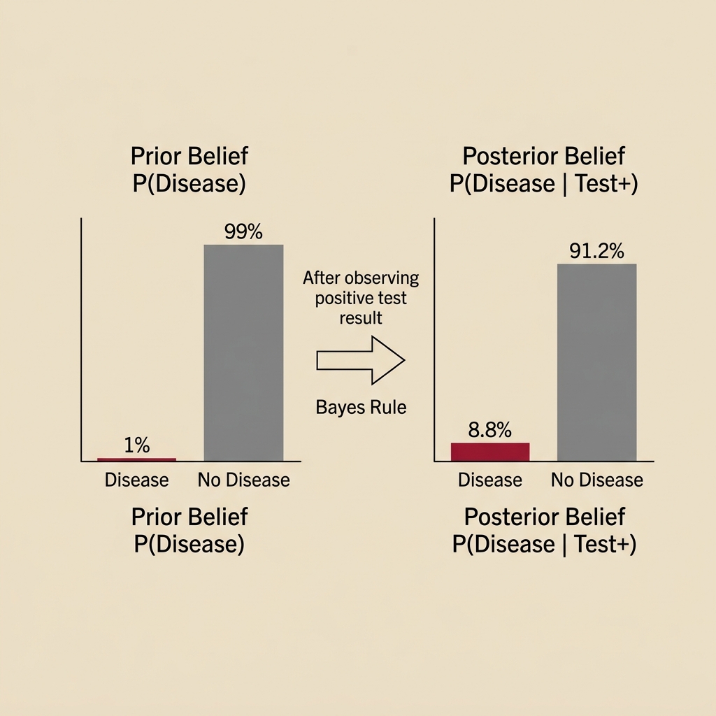
\[P(D \mid T^+) = \frac{0.95 \times 0.01}{0.1085} = \frac{0.0095}{0.1085} \approx 0.0876\]
Result: \(P(D \mid T^+) \approx\) 8.8%. Even with a “highly accurate” test, a positive result means only an 8.8% chance of disease!
Why Is the Posterior So Low?
This surprises most students. The answer lies in the base rate (prior probability).
Think about 10,000 people:
- 100 have the disease (1%)
- 9,900 are healthy
Among the 100 sick: 95 test positive
Among the 9,900 healthy: 990 test positive (false positives!)
Total positive tests: \(95 + 990 = 1{,}085\)
Truly sick among positives: \(95 / 1{,}085 = 8.8\%\)
When the disease is rare, even a good test produces many false positives that overwhelm the true positives.
TABLE OF CONTENTS
Watch Out for These Pitfalls
Confusion 1: \(P(A \mid B) \neq P(B \mid A)\)
The probability of disease given a positive test is NOT the same as the probability of a positive test given disease.
Confusion 2: Independent ≠ Mutually Exclusive
Independent events CAN happen together. Mutually exclusive events CANNOT.
Confusion 3: Conditioning changes the sample space
\(P(A \mid B)\) is about a different universe than \(P(A)\), one where \(B\) is known to have happened.
Confusion 4: Bayes rule is not just a formula
It is a reasoning framework: update your belief using evidence. This is the foundation of probabilistic AI.
Check Your Understanding
If a test is highly accurate, does a positive result always mean the patient probably has the disease? No. If the disease is rare, false positives can dominate.
Are “rain today” and “not rain today” independent? No. They are mutually exclusive (and complementary).
If two events are mutually exclusive, can they be independent? No (unless one has zero probability). \(P(A \cap B)=0 \neq P(A)P(B)\).
What is the difference between \(P(D \mid T)\) and \(P(T \mid D)\)? \(P(D \mid T)\) = disease given positive test. \(P(T \mid D)\) = positive test given disease. Different!
Summary
| Concept | Key Takeaway |
|---|---|
| Sample Space & Events | Probability assigns numbers to events (sets of outcomes) |
| Probability Rules | Axioms, complement, addition rule: the building blocks |
| Conditional Probability | \(P(A \mid B) = P(A \cap B) / P(B)\): how evidence changes probability |
| Independence | \(P(A \cap B) = P(A)P(B)\); knowing one event gives no info about the other |
| Bayes Rule | \(P(A \mid B) = P(B \mid A)P(A)/P(B)\): update belief from prior + evidence |
Thank You!


![]()
The University of Alabama