CS-466/566: Math for AI
Module 03: Linear Regression
2026-03-23
Linear Regression
Can you design a linear road that pass by all these houses equally?!

Linear Regression
Can you design a linear road that pass by all these houses equally?!

Housing Prices Problem
- What are the features and labels here?
- Is it classification or regression problem?
- What is the price of the house of 4 rooms?
- What is the price per extra room? (#Room \(\times\) weight)
- What is the base price? (Bias)
- What is the equation that represents the price?
- Price = 100 + 50 * (#Rooms)

How machines learn it? [Remember-Formulate-Predict]

How machines learn it? [Remember-Formulate-Predict]
Linear Regression
Price = 100 + 50 * (#Rooms)
Slope
Measures how steep the line is.
Y-intercept
It is the height at which the line crosses the vertical (y) axis.

Linear Equation
Linear Equation is the equation of a line. \(y=mx+b\)
How many lines can solve the problem?
How machines learn it? [Remember-Formulate-Predict]
Price = 100 + 50 \(\times\) (#Rooms)
Price = 100 + 50 \(\times\) (4) = 300
Some Questions:
- Can we have multiple features data?
- How does computer learn this equation?

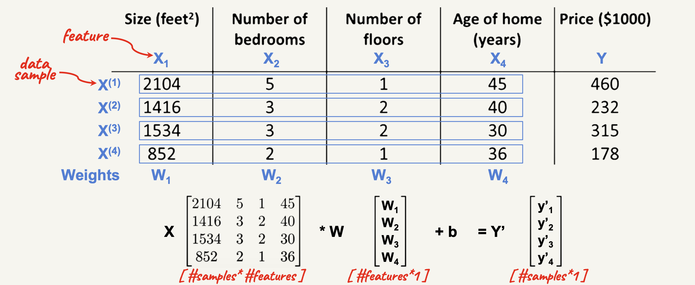
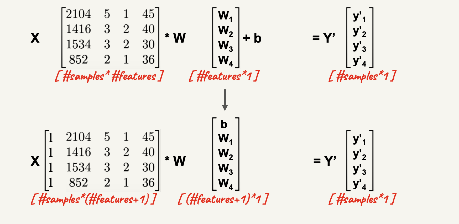
Multivariate Linear Regression
Price = 30 * (#Rooms) + 1.5 * (Size) + 10 * (Schools Quality) - 2 * (Age) + 50
- 1 bias and multiple weights
- Different sign of weights
- Different weights value
- What is the shape of the model? Still linear?

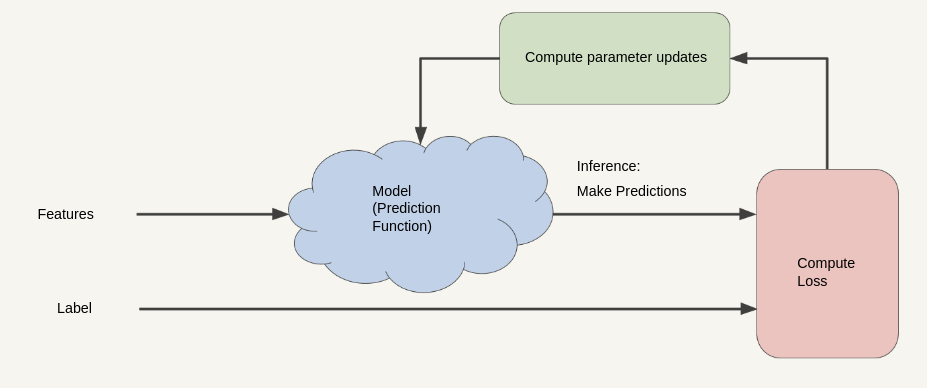
How machines formulate this equation? [Overview]


Training and Loss
- Training a model simply means learning (determining) good values for all the weights and the bias from labeled examples.
- Loss is the penalty for a bad prediction.
- Perfect prediction means the loss is zero.
- Bad model have large loss.
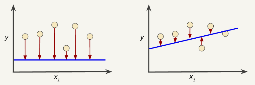
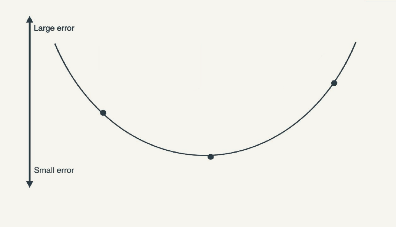
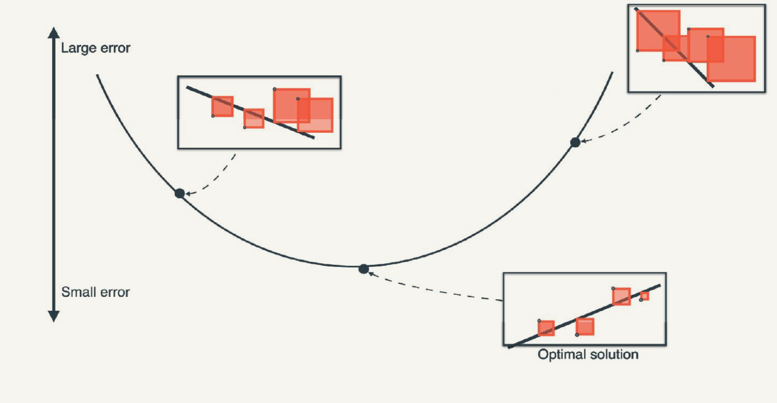
Suppose we selected the following weights and biases. Which of them have lower loss?
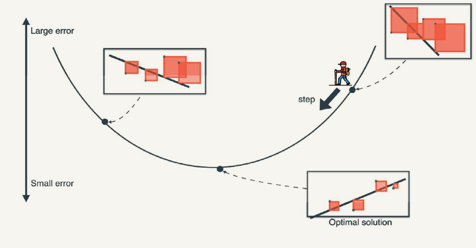
Reducing Loss
- Training is a feedback iterative process that uses the loss function to improve the model parameters.
Some Questions: - How to define loss to measure the performance of the model? - What initial values should we set for \(w_1\) and \(w_0\)? - How to update \(w_1\) and \(w_0\)?
Loss Definition
Which model is better and why? Which model have a lower loss?

Absolute Loss (L1 Loss)
The absolute loss is the sum of the absolute differences between the observed and predicted values.

\(| \text{observation}(x) - \text{prediction}(x) | = |(y-y')|\)
Absolute Loss (L1 Loss)
The absolute loss is the sum of the absolute differences between the observed and predicted values.

Squared Loss (L2 Loss)
The squared loss is the sum of the squared differences between the observed and predicted values.

\([ \text{observation}(x) - \text{prediction}(x) ]^2 = [(y-y')]^2\)
Squared Loss (L2 Loss)
The squared loss is the sum of the squared differences between the observed and predicted values.

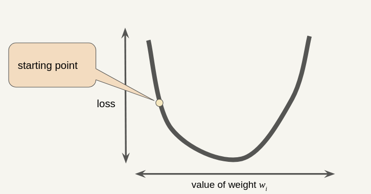
Gradient Descent (Recap)
Note that a gradient is a vector, so it has both of the following characteristics: - Magnitude - Direction
The gradient descent algorithm takes a step in the direction of the negative gradient.
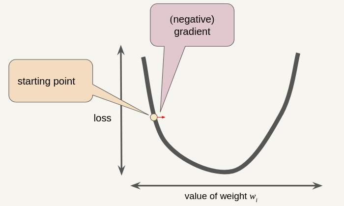
The gradient descent algorithm adds some fraction of the gradient’s magnitude (Learning Rate \(\eta\)) to the previous point.
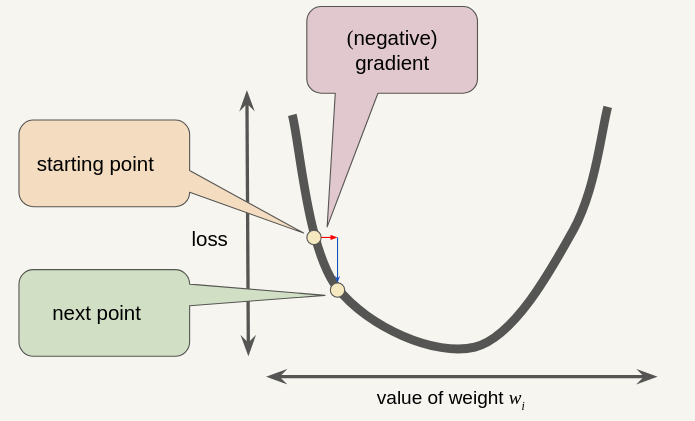
\[ w_{new} = w_{old} - \eta \cdot \frac{d\ \text{loss}}{dw} \]
Gradient Descent for Linear Regression
Learning Rate
- Gradient descent algorithms multiply the gradient by a scalar known as the learning rate (also sometimes called step size).
- How can we choose the learning rate?
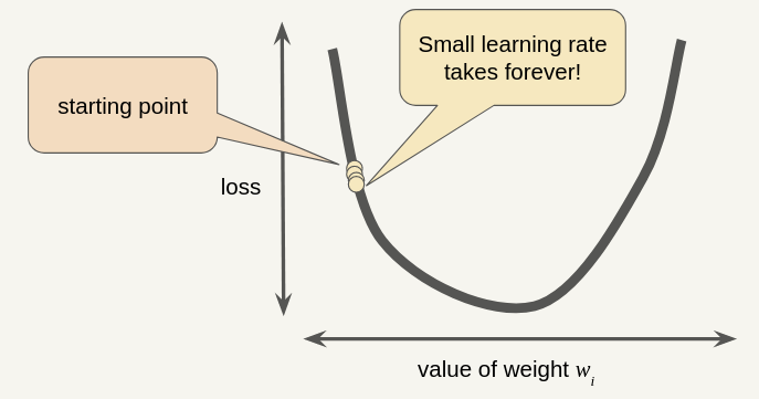
Small Learning Rate
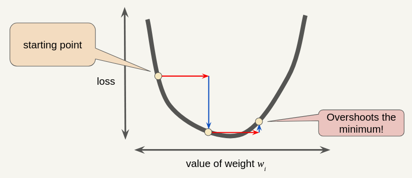
Large Learning Rate
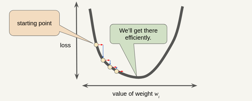
Optimal Learning Rate (usually 0.01)
Multivariate Output Visualization
The Normal Equation
Thank You!