CS-466/566: Math for AI

Module 02: Multivariate Calculus

Dr. Mahmoud Mahmoud

The University of Alabama

2026-03-23

TABLE OF CONTENTS

1. Functions
2. Derivatives
3. Calculus Toolbox: Rules & Special Cases
4. Multivariate Calculus

What is a Function?

  • A function maps a set of inputs to an output.
  • Notation: \(f(x)\) denotes the output of function \(f\) for input \(x\).
  • Choosing a function to model a system is the “creative essence of science.”

%%{init: {'theme': 'base', 'themeVariables': { 'fontSize': '37px', 'fontFamily': 'arial' }}}%%
graph LR
    X["X, Y, Z, T"]
    B["Function f"]
    Y["Y, W, V"]

    X --> B
    B --> Y

    style B fill:#f3e5f5,stroke:#333,stroke-width:3px
    style X fill:none,stroke:none
    style Y fill:none,stroke:none

Function as a transformation from input to output

Function Examples

Linear Functions:

  • \(f(x) = mx + b\) (straight line)
  • \(f(x) = 2x + 3\)

Quadratic Functions:

  • \(f(x) = ax^2 + bx + c\) (parabola)
  • \(f(x) = x^2 - 4x + 4\)

Trigonometric Functions:

  • \(f(x) = \sin(x)\) (sine wave)
  • \(f(x) = \cos(x)\) (cosine wave)

Multivariate Functions:

  • \(f(x,y) = x^2 + y^2\) (paraboloid)
  • \(f(x,y,z) = x + y + z\) (plane)

Function Visualizations (1/2)

Function Visualizations (2/2)

TABLE OF CONTENTS

1. Functions
2. Derivatives
3. Calculus Toolbox: Rules & Special Cases
4. Multivariate Calculus

Introduction to Derivatives

Leibniz Lagrange Newton Euler

\(\frac{dy}{dx}\)

\(y'(x)\)

\(\dot{y}\)

\(D_x y\)

Interactive Derivative Visualization

The derivative at point \(x\) is defined as:

\[f'(x) = \lim_{\Delta x \to 0} \frac{f(x + \Delta x) - f(x)}{\Delta x}\]

Interactive Features:

  • Adjust \(\Delta x\) to see how the secant line changes
  • Move the point \(x\) to explore different locations
  • Choose different functions to visualize
  • Watch the rise/run calculation update in real-time

TABLE OF CONTENTS

1. Functions
2. Derivatives
3. Calculus Toolbox: Rules & Special Cases
4. Multivariate Calculus

Derivative of a Linear Function: Step-by-Step

For any function \(f(x)\), the derivative at a point \(x\) is: \[f'(x) = \lim_{\Delta x \to 0} \frac{f(x+\Delta x) - f(x)}{\Delta x}\]

Example: \(f(x) = 3x + 2\)

  1. Compute \(f(x + \Delta x)\): \[f(x+\Delta x) = 3(x+\Delta x) + 2 = 3x + 3\Delta x + 2\]
  1. Form the difference quotient: \[\frac{[3x + 3\Delta x + 2] - [3x + 2]}{\Delta x} = \frac{3\Delta x}{\Delta x} = 3\]

Derivative of a Quadratic Function

Example: \(f(x) = 5x^2\)

  1. Compute \(f(x + \Delta x)\): \[\begin{align*} f(x+\Delta x) &= 5(x+\Delta x)^2 \\ &= 5(x^2 + 2x\Delta x + (\Delta x)^2) \\ &= 5x^2 + 10x\Delta x + 5(\Delta x)^2 \end{align*}\]
  1. Form the difference quotient: \[\begin{align*} \frac{[5x^2 + 10x\Delta x + 5(\Delta x)^2] - [5x^2]}{\Delta x} &= \frac{10x\Delta x + 5(\Delta x)^2}{\Delta x} = 10x + 5\Delta x \end{align*}\]
  1. Take the limit as \(\Delta x \to 0\): \[\lim_{\Delta x \to 0} (10x + 5\Delta x) = 10x\]

1. The Sum Rule

  • Sum Rule: The derivative of a sum is the sum of the derivatives.
  • Intuition: If you add two functions, their rates of change simply add together.

\[ \frac{d}{dx}[f(x) + g(x)] = f'(x) + g'(x) \]

2. Power Rule

  • Statement: The derivative of \(x^n\) with respect to \(x\) is \(nx^{n-1}\).
  • Intuition: The exponent “comes down” as a multiplier, and the new exponent is one less than before.

\[ \frac{d}{dx} x^n = n x^{n-1} \]

Example 1:
Let \(f(x) = x^4 \implies f'(x) = 4x^{3}\)

Example 2:
Let \(f(x) = 7x^3 \implies f'(x) = 7 \cdot 3x^{2} = 21x^{2}\)

3. Product Rule

The product rule is a formula used to find the derivative of a product of two functions. If \(A(x) = f(x)g(x)\), then the derivative \(A'(x)\) is:

\[A'(x) = f'(x)g(x) + f(x)g'(x)\]
(First times derivative of the second, plus second times derivative of the first)

Example: \(h(x) = x^2 \sin(x)\)

  • Let \(f(x) = x^2 \implies f'(x) = 2x\)
  • Let \(g(x) = \sin(x) \implies g'(x) = \cos(x)\)
  • \(h'(x) = (2x)\sin(x) + (x^2)\cos(x)\)

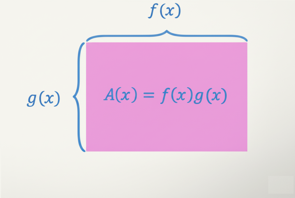
3. Product Rule Geometric Proof

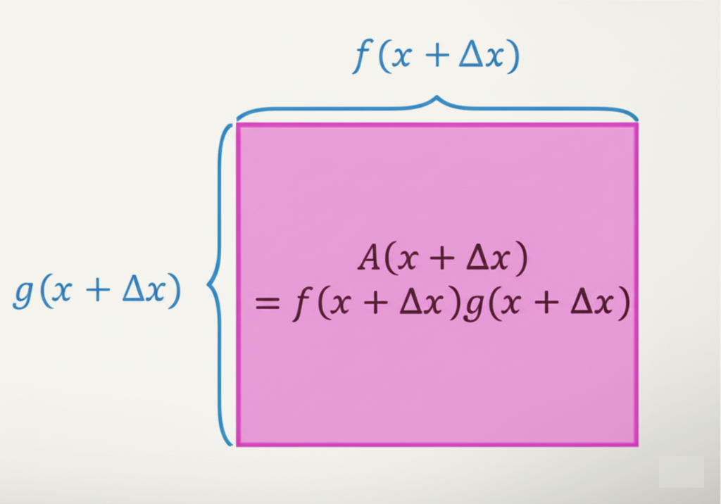
Let \(A(x) = f(x)g(x)\) represent the area of a rectangle. A small change \(\Delta x\) increases this area by \(\Delta A(x)\), added in three regions:

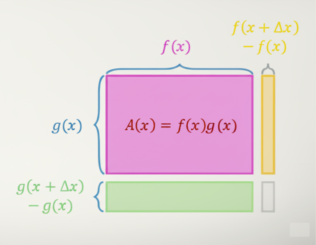
  1. Right strip: \(g(x)[f(x+\Delta x) - f(x)]\)
  2. Top strip: \(f(x)[g(x+\Delta x) - g(x)]\)
  3. Corner: \([f(x+\Delta x) - f(x)][g(x+\Delta x) - g(x)]\) (vanishes as \(\Delta x \to 0\))

Total change in area: \[ \Delta A(x) = f(x)\Delta g + g(x)\Delta f + (\Delta f)(\Delta g) \]

Divide by \(\Delta x\) and take the limit: \[ A'(x) = f(x)g'(x) + g(x)f'(x) \]

4. Chain Rule

%%{init: {'theme': 'base', 'themeVariables': { 'fontSize': '29px', 'fontFamily': 'arial' }}}%%
graph LR
    X["x"] --> F["f(x)"]
    F --> G["g(u)"]
    
    style X fill:#e1f5fe
    style F fill:#f3e5f5
    style G fill:#e8f5e8

\[ \frac{d}{dx}[g(f(x))] = g'(f(x)) \cdot f'(x) \]

Note: The rate of change of the composition is the product of the rates of change of the individual functions. This effect due to the accumulation of the changes.

Chain Rule Example:

Let \(h(x) = g(f(x))\). If \(f'(x) = 3\) and \(g'(u) = 10\):

\[h'(x) = g'(f(x)) \cdot f'(x) = 10 \cdot 3 = 30\]

Chain Rule Practice (1/2)

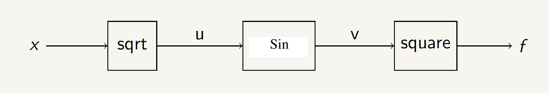
  1. Write the nested function in math notation: \(f(x) = \, ??\)
  2. Assume \(x=2\), compute \(u\), \(v\), and \(f\)
  3. Compute \(\frac{\partial f}{\partial x}\big|_{x=2}\) using the finite difference rule and the nested function notation you wrote. \[ \frac{df}{dx}\Big|_{x=a} = \frac{f(a+\triangle) + f(a-\triangle)}{2\triangle} \]
  4. Write the formula for the chain rule \(\frac{\partial f}{\partial x}\big|_{x=2}\) and use it to compute the derivative again and verify you get the same answer.

Chain Rule Practice (2/2)

1. Math notation:
\[f(x) = (\mathrm{sigmoid}(\sqrt{x}))^2\]

2. Computing values at \(x=2\): \[\begin{align*} u &= \sqrt{2} \approx 1.414 \\ v &= \sin(1.414) \approx 0.987 \\ f &= (0.987)^2 \approx 0.974 \end{align*}\]

3. Using the finite difference rule with \(\triangle = 0.001\): \[\begin{align*} \frac{\partial f}{\partial x}\Big|_{x=2} = \frac{f(2.001) - f(1.999)}{0.002} \approx 0.135 \end{align*}\]

4. Using chain rule: \[\begin{align*} \frac{\partial f}{\partial x} = \frac{\partial f}{\partial v} \cdot \frac{\partial v}{\partial u} \cdot \frac{\partial u}{\partial x} \implies 2(0.987) \cdot 0.156 \cdot 0.354 \approx 0.109 \end{align*}\]

The Power of Chain Rule in Deep Learning

Why not use the finite difference to compute derivatives?
  • Computationally expensive and almost impossible to get a closed-form expression for complicated neural network weights.
  • The chain rule is the most important tool we have for computing derivatives in deep learning (Backpropagation).
  • The chain rule for updating early layer weights shares most of its computation with the chain rule for updating later layer weights.

TABLE OF CONTENTS

1. Functions
2. Derivatives
3. Calculus Toolbox: Rules & Special Cases
4. Multivariate Calculus

Multiple Inputs, Single Output

Multiple Inputs Single Output Diagram

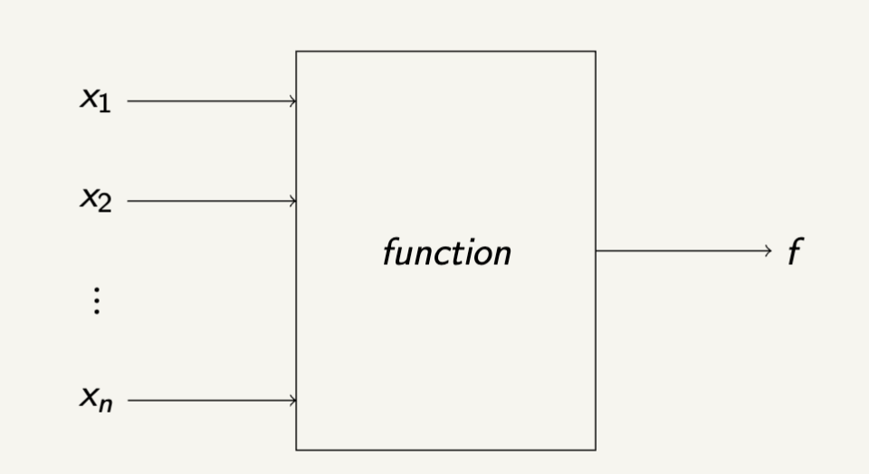
  • Setup: \(n\) inputs (\(x_1, x_2, \ldots, x_n\)), one output \(f\).
  • Question: How do we compute the derivative of the output with respect to each input?

Derivative of Functions with Multiple Inputs

Multiple Inputs Single Output Diagram

  • The derivative of the output with respect to the inputs is a vector of partial derivatives:

\[ \frac{\partial f}{\partial x} = \left[ \frac{\partial f}{\partial x_1}, \frac{\partial f}{\partial x_2}, \dots, \frac{\partial f}{\partial x_n} \right] \]

  • This vector is called the gradient of \(f\) with respect to \(x\). The output \(f\) changes by a small amount \(\Delta f\) when any input \(x_i\) changes by a small amount \(\Delta x_i\).

Example: Gradient of a Simple Function

Let \(f(x_1, x_2) = x_1^2 + x_2^2\).
The gradient is: \[ \nabla f = \left[ \frac{\partial f}{\partial x_1}, \frac{\partial f}{\partial x_2} \right] = [2x_1, 2x_2] \]

Gradient Example Diagram

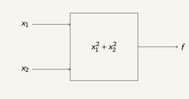
At point \((x_1, x_2) = (3, 4)\): \[\begin{align*} \frac{\partial f}{\partial x_1} &= 2x_1 = 2(3) = 6 \\ \frac{\partial f}{\partial x_2} &= 2x_2 = 2(4) = 8 \end{align*}\]

Numerical approximation at \((3,4)\):

  • \(\frac{f(3.001, 4) - f(3, 4)}{0.001} \approx 6\)
  • \(\frac{f(3, 4.001) - f(3, 4)}{0.001} \approx 8\)

Function Contours

Contour lines show where \(f(x_1, x_2) = x_1^2 + x_2^2\) has constant values.

  • Contours are like the projections of the function on the a plane
  • The function increases as you move outward.

Vector-Field: Gradient of a Function

Left is \(f(x_1, x_2) = x_1^2 + x_2^2\). Right is the gradient \(\nabla f = [2x_1, 2x_2]\)

  • Direction: Vectors point away from the origin (0,0) - the direction of steepest increase
  • Magnitude: Vectors get longer as you move away from the origin

Complex Function Visualization

Function: \(z(x, y) = 3(1-x)^2 e^{-x^2-(y+1)^2} - 10\left(\frac{x}{5} - x^3 - y^5\right)e^{-x^2-y^2} - \frac{1}{3}e^{-(x+1)^2-y^2}\)

Left: 3D surface showing the complex terrain
Right: Heat plot showing the same function in 2D with color intensity

Gradient Vector Field

Gradient: \(\nabla z = \left[\frac{\partial z}{\partial x}, \frac{\partial z}{\partial y}\right]\)

Gradient vectors are perpendicular to contour lines and point “uphill”!

Jacobian Matrix

Function with Multiple Inputs and Outputs:

Multiple Inputs Single Output Diagram

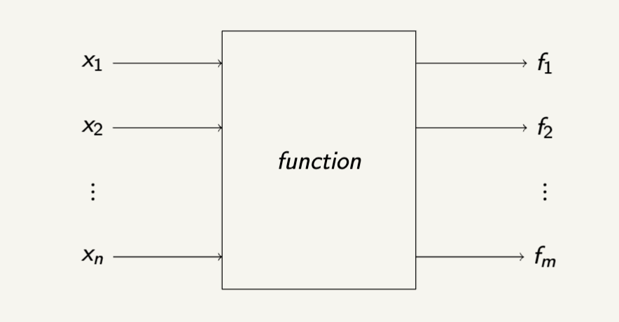
For functions with multiple outputs, the derivative becomes a matrix called the Jacobian matrix (J):

\[\begin{bmatrix} \frac{\partial f_1}{\partial x_1} & \frac{\partial f_1}{\partial x_2} & \cdots & \frac{\partial f_1}{\partial x_n} \\ \frac{\partial f_2}{\partial x_1} & \frac{\partial f_2}{\partial x_2} & \cdots & \frac{\partial f_2}{\partial x_n} \\ \vdots & \vdots & \ddots & \vdots \\ \frac{\partial f_m}{\partial x_1} & \frac{\partial f_m}{\partial x_2} & \cdots & \frac{\partial f_m}{\partial x_n} \end{bmatrix}\]

Example: Jacobian Matrix

Let \(f(x, y, z) = x^2 \cdot y + 3z\).

The Jacobian matrix is a vector of partial derivatives: \[\nabla f = \left[ \frac{\partial f}{\partial x}, \frac{\partial f}{\partial y}, \frac{\partial f}{\partial z} \right]\]

Calculating the partial derivatives: - \(\frac{\partial f}{\partial x} = 2x \cdot y\) (treat y and z as constants) - \(\frac{\partial f}{\partial y} = x^2\) (treat x and z as constants)
- \(\frac{\partial f}{\partial z} = 3\) (treat x and y as constants)

Therefore: \[\nabla f = [2xy, x^2, 3]\]

At point (2, 1, 0): \[\nabla f(2, 1, 0) = [4, 4, 3]\]

Thank You!