CS-466/566: Math for AI

Module 02: Computational Linear Algebra-2

Dr. Mahmoud Mahmoud

The University of Alabama

2026-03-23

TABLE OF CONTENTS

1. Introduction●

2. Matrix Multiplication○

3. Matrix Properties○

• What is the Determinant?

• What is a Matrix Inverse?

• What is Matrix Rank?

7. Change of Basis○

8. Solving Linear Systems○

What is a Matrix?

1. The “Data” Perspective (CS):

A matrix is just a 2D array (table) of numbers.

\[ X = \begin{bmatrix} \text{age} & \text{height} \\ 25 & 180 \\ 30 & 165 \\ 42 & 175 \end{bmatrix} \]

• Rows: Samples (people)
• Columns: Features (attributes)

2. The “Math” Perspective:

A matrix is a function or transformation.

• It acts on vectors: \(f(\mathbf{x}) = A\mathbf{x}\)
• It warps space (stretches, rotates, shears).

We will focus on the Math Perspective today.

Matrices as Basis Changers (1/2)

1. The Standard World (Identity)

\[ I = [\mathbf{e}_1 | \mathbf{e}_2] = \begin{bmatrix} 1 & 0 \\ 0 & 1 \end{bmatrix} \]

A vector \(\mathbf{x} = (2, 2)\) means: \[ \mathbf{x} = 2\mathbf{e}_1 + 2\mathbf{e}_2 = 2\begin{bmatrix} 1 \\ 0 \end{bmatrix} + 2\begin{bmatrix} 0 \\ 1 \end{bmatrix} = \begin{bmatrix} 2 \\ 2 \end{bmatrix} \]

Result: You land exactly where you expect, at \((2,2)\).

Matrices as Basis Changers (2/2)

2. The Transformed World

\[ A = [\mathbf{v}_1 | \mathbf{v}_2] = \begin{bmatrix} 2 & 0 \\ 0 & 0.5 \end{bmatrix} \]

The same coordinates \((2, 2)\) now mean: \[ A\mathbf{x} = 2\mathbf{v}_1 + 2\mathbf{v}_2 = 2\begin{bmatrix} 2 \\ 0 \end{bmatrix} + 2\begin{bmatrix} 0 \\ 0.5 \end{bmatrix} \] \[ = \begin{bmatrix} 4 \\ 0 \end{bmatrix} + \begin{bmatrix} 0 \\ 1 \end{bmatrix} = \begin{bmatrix} 4 \\ 1 \end{bmatrix} \]

Result: The numbers (2,2) now land you at the physical location \((4, 1)\).

Matrix-Vector Multiplication is just a Linear Combination of Columns.

Matrix-Vector Multiplication: The Mechanics

The mechanics of matrix-vector multiplication can be visualized in two ways:

Column View

\[\begin{bmatrix} \color{red}{1} & \color{blue}{2} & \color{green}{3} \\ \color{red}{4} & \color{blue}{5} & \color{green}{6} \\ \color{red}{7} & \color{blue}{8} & \color{green}{9} \end{bmatrix} \begin{bmatrix} \color{red}{2} \\ \color{blue}{1} \\ \color{green}{0} \end{bmatrix}\]

\[= \color{red}{2}\begin{bmatrix} 1 \\ 4 \\ 7 \end{bmatrix} + \color{blue}{1}\begin{bmatrix} 2 \\ 5 \\ 8 \end{bmatrix} + \color{green}{0}\begin{bmatrix} 3 \\ 6 \\ 9 \end{bmatrix} = \begin{bmatrix} 4 \\ 13 \\ 22 \end{bmatrix}\]

Row View (Dot Products)

Row 1: \([1,2,3] \cdot [2,1,0] = 4\)

Row 2: \([4,5,6] \cdot [2,1,0] = 13\)

Row 3: \([7,8,9] \cdot [2,1,0] = 22\)

\[\Rightarrow \begin{bmatrix} 4 \\ 13 \\ 22 \end{bmatrix}\]

Both views give the same result — use whichever is more intuitive!

Types of Matrix Transformations

Type	Matrix	Effect	Example: \(A \times (2,2)^T\)
Identity	\(\begin{pmatrix} 1 & 0 \\ 0 & 1 \end{pmatrix}\)	No change	\(\begin{pmatrix} 1 & 0 \\ 0 & 1 \end{pmatrix}\begin{pmatrix} 2 \\ 2 \end{pmatrix} = \begin{pmatrix} 2 \\ 2 \end{pmatrix}\)
Scaling	\(\begin{pmatrix} 2 & 0 \\ 0 & 3 \end{pmatrix}\)	Stretch	\(\begin{pmatrix} 2 & 0 \\ 0 & 3 \end{pmatrix}\begin{pmatrix} 2 \\ 2 \end{pmatrix} = \begin{pmatrix} 4 \\ 6 \end{pmatrix}\)
Shear	\(\begin{pmatrix} 1 & 1 \\ 0 & 1 \end{pmatrix}\)	Slant	\(\begin{pmatrix} 1 & 1 \\ 0 & 1 \end{pmatrix}\begin{pmatrix} 2 \\ 2 \end{pmatrix} = \begin{pmatrix} 4 \\ 2 \end{pmatrix}\)
Reflection	\(\begin{pmatrix} -1 & 0 \\ 0 & 1 \end{pmatrix}\)	Flip	\(\begin{pmatrix} -1 & 0 \\ 0 & 1 \end{pmatrix}\begin{pmatrix} 2 \\ 2 \end{pmatrix} = \begin{pmatrix} -2 \\ 2 \end{pmatrix}\)
Rotation 90°	\(\begin{pmatrix} 0 & -1 \\ 1 & 0 \end{pmatrix}\)	Rotate	\(\begin{pmatrix} 0 & -1 \\ 1 & 0 \end{pmatrix}\begin{pmatrix} 2 \\ 2 \end{pmatrix} = \begin{pmatrix} -2 \\ 2 \end{pmatrix}\)

Combining transformations: \(C = BA\) applies \(A\) first, then \(B\)

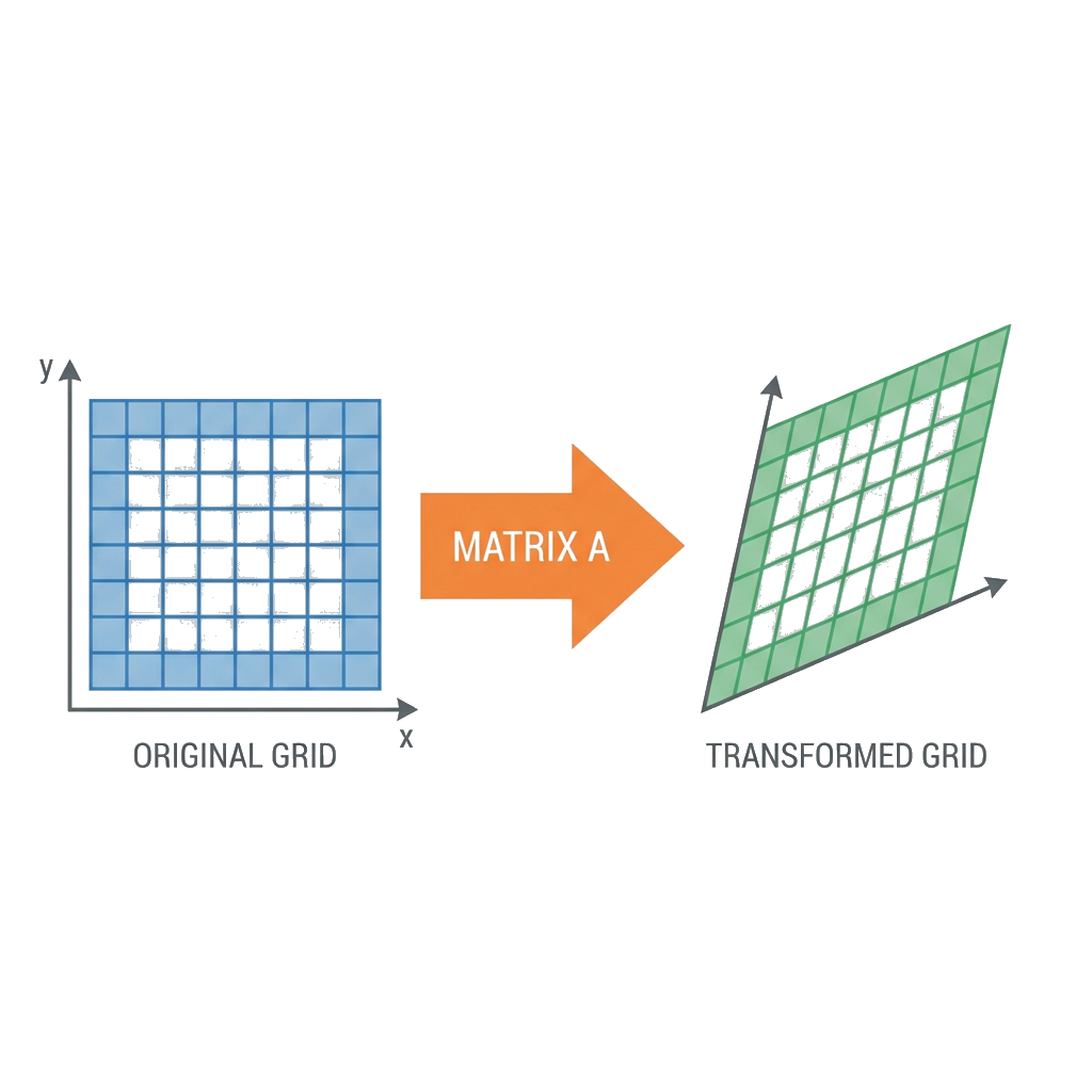
Matrix Columns = Transformed Basis Vectors

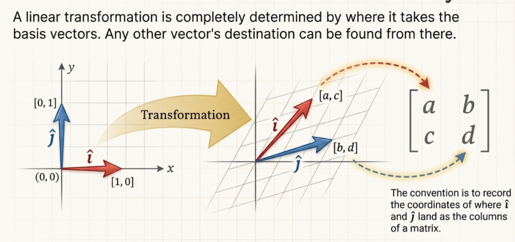
The columns of a matrix tell you where \(\hat{i}\) and \(\hat{j}\) land!

Matrix Transformations in Action

Matrix columns show where basis vectors \(\hat{i}\) and \(\hat{j}\) land after the transformation!

TABLE OF CONTENTS

1. Introduction✓

2. Matrix Multiplication●

3. Matrix Properties○

• What is the Determinant?

• What is a Matrix Inverse?

• What is Matrix Rank?

7. Change of Basis○

8. Solving Linear Systems○

What is Matrix Multiplication?

\(A\) acts on each column of \(B\) to produce each column of \(C\)

\[ A \cdot B = A \cdot \begin{bmatrix} \mathbf{b}_1 & \mathbf{b}_2 & \cdots & \mathbf{b}_n \end{bmatrix} = \begin{bmatrix} A\mathbf{b}_1 & A\mathbf{b}_2 & \cdots & A\mathbf{b}_n \end{bmatrix} = C \]

Example: \[ \begin{pmatrix} 2 & 0 \\ 0 & 3 \end{pmatrix} \begin{pmatrix} 1 & 0 \\ 0 & 1 \end{pmatrix} = \begin{pmatrix} A \cdot \begin{pmatrix} 1 \\ 0 \end{pmatrix} & A \cdot \begin{pmatrix} 0 \\ 1 \end{pmatrix} \end{pmatrix} = \begin{pmatrix} 2 & 0 \\ 0 & 3 \end{pmatrix} \] Each column of the identity is transformed by the scaling matrix!

Matrix multiplication = applying the left matrix to each column of the right matrix.

Matrix Multiplication: The Mechanics

Computing \((AB)_{ij}\):

\[c_{ij} = \sum_{k=1}^{n} a_{ik} \cdot b_{kj}\]

Steps:

1. Take row \(i\) from \(A\)
2. Take column \(j\) from \(B\)
3. Dot product → element \((i,j)\) of \(C\)

Dimension rule: \[(m \times n) \cdot (n \times p) = (m \times p)\]

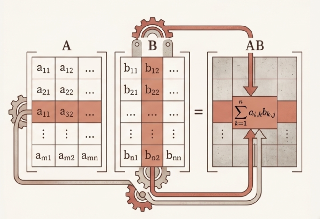
Row of \(A\) meets Column of \(B\) → one element of \(AB\)

Exercise: Matrix Multiplication

Calculate \(C = A \times B\):

\[ \underbrace{\begin{bmatrix} 1 & 2 & 1 \\ 0 & 1 & 0 \end{bmatrix}}_{2 \times 3} \times \underbrace{\begin{bmatrix} 1 & 0 \\ 0 & 1 \\ 1 & 2 \end{bmatrix}}_{3 \times 2} \]

1. What are the dimensions of the output matrix \(C\)?

Answer: \(2 \times 2\)

(Inner dimensions 3 match; Outer dimensions \(2 \times 2\) remain)

2. What is the result matrix \(C\)?

Answer: \[ \begin{bmatrix} 2 & 4 \\ 0 & 1 \end{bmatrix} \]

Matrix Multiplication: Function Composition - Order Matters

Scale then Rotate (left): \(RS = \underbrace{\begin{pmatrix} 0.7 & -0.7 \\ 0.7 & 0.7 \end{pmatrix}}_{R} \underbrace{\begin{pmatrix} 2 & 0 \\ 0 & 0.5 \end{pmatrix}}_{S} = \begin{pmatrix} 1.4 & -0.35 \\ 1.4 & 0.35 \end{pmatrix}\)

Rotate then Scale (right): \(SR = \underbrace{\begin{pmatrix} 2 & 0 \\ 0 & 0.5 \end{pmatrix}}_{S} \underbrace{\begin{pmatrix} 0.7 & -0.7 \\ 0.7 & 0.7 \end{pmatrix}}_{R} = \begin{pmatrix} 1.4 & -1.4 \\ 0.35 & 0.35 \end{pmatrix}\)

Machine Learning Connection: Neural Networks

In Deep Learning, each layer of a Neural Network is just a matrix multiplication (plus a non-linearity).

• The matrix warps the space (shears, rotates, stretches).
• The goal? Transform “tangled” data into a space where it is linearly separable (easy to classify).

TABLE OF CONTENTS

1. Introduction✓

2. Matrix Multiplication✓

3. Matrix Properties●

• What is the Determinant?

• What is a Matrix Inverse?

• What is Matrix Rank?

7. Change of Basis○

8. Solving Linear Systems○

What is the Determinant?

Watch how different transformations change the area of the unit square!

What is the Determinant?

The determinant measures how much a transformation scales area.

For a 2×2 matrix: \[\det\begin{pmatrix} a & b \\ c & d \end{pmatrix} = ad - bc\]

Geometric Meaning:

• Start with a unit square (area = 1)
• Apply matrix transformation
• New area = \(|\det(A)|\)

Quick Examples:

Matrix	det	Area Factor
\(\begin{pmatrix} 2 & 0 \\ 0 & 3 \end{pmatrix}\)	6	6× bigger
\(\begin{pmatrix} 1 & 1 \\ 0 & 1 \end{pmatrix}\)	1	Same area
\(\begin{pmatrix} 2 & 4 \\ 1 & 2 \end{pmatrix}\)	0	Collapsed!

The determinant tells you how the transformation scales space!

What the Sign Tells Us

det > 0

✅ Orientation Preserved

The “handedness” stays the same (counterclockwise stays counterclockwise)

det < 0

🔄 Orientation Flipped

Like looking in a mirror — left becomes right

det = 0

💀 Space Collapsed

2D → 1D line (or point). Matrix is singular — no inverse!

det = 0 means the transformation loses information — you can’t undo it!

Computing Determinants in NumPy

import numpy as np

#> Define matrices
A = np.array([[2, 0], 
              [0, 3]])    # Scaling matrix

B = np.array([[1, 2], 
              [3, 4]])    # General matrix

C = np.array([[2, 4], 
              [1, 2]])    # Singular matrix (det = 0)

#> Compute determinants
print(f"det(A) = {np.linalg.det(A):.2f}")  #> Expected: 6
print(f"det(B) = {np.linalg.det(B):.2f}")  #> Expected: -2
print(f"det(C) = {np.linalg.det(C):.2f}")  #> Expected: 0

det(A) = 6.00
det(B) = -2.00
det(C) = 0.00

Use np.linalg.det(A) to compute the determinant of any matrix!

Exercise: Determinants

Calculate the determinant of \(M = \begin{pmatrix} 3 & 2 \\ 1 & 4 \end{pmatrix}\).

1. Compute \(\det(M) = ad - bc\):

Answer: 10

(\(3(4) - 2(1) = 12 - 2 = 10\))

2. Geometric Interpretation:

Answer: Area scales by 10x

The unit square becomes a parallelogram with area 10.

Exercise: Determinant

Are the vectors \(\mathbf{v}_1 = \begin{pmatrix} 1 \\ 2 \end{pmatrix}\) and \(\mathbf{v}_2 = \begin{pmatrix} 2 \\ 4 \end{pmatrix}\) linearly independent? Use the determinant!

1. Form Matrix & Compute Det:

\(\det\begin{pmatrix} 1 & 2 \\ 2 & 4 \end{pmatrix} = 1(4) - 2(2) = 0\)

2. Conclusion:

Linearly Dependent!

Since \(\det = 0\), the “area” is zero. The vectors lie on the same line (they are parallel).

What is a Matrix Inverse?

The inverse \(A^{-1}\) “undo” the transformation \(A\): \[A A^{-1} = A^{-1} A = I\]

Geometric Intuition

• Rotation: Rotate \(30^\circ\) \(\to\) Rotate \(-30^\circ\)
• Scaling: Scale by \(2\) \(\to\) Scale by \(0.5\)
• Shear: Shear right \(\to\) Shear left

2×2 Inverse Formula

\[A^{-1} = \frac{1}{\det(A)} \begin{pmatrix} d & -b \\ -c & a \end{pmatrix}\]

Swap \(a,d\) | Negate \(b,c\) | Divide by \(\det\)

The inverse only exists when \(\det(A) \neq 0\)!

Matrix Inverse: Example

Given: \[A = \begin{pmatrix} 3 & 1 \\ 2 & 4 \end{pmatrix}\]

Step 1: Calculate determinant \[\det(A) = 3 \times 4 - 1 \times 2 = 12 - 2 = 10\]

Step 2: Apply the formula (swap, negate, divide) \[A^{-1} = \frac{1}{10} \begin{pmatrix} 4 & -1 \\ -2 & 3 \end{pmatrix} = \begin{pmatrix} 0.4 & -0.1 \\ -0.2 & 0.3 \end{pmatrix}\]

Step 3: Verify: \(A \cdot A^{-1} = I\)

Always verify your inverse by checking that \(A \cdot A^{-1} = I\)!

Computing Inverses in NumPy

import numpy as np
#> Define a matrix  
A = np.array([[3, 1], 
              [2, 4]])
#> Compute inverse
A_inv = np.linalg.inv(A)
print("\nA^(-1) =\n", A_inv)

#> Verify: A @ A_inv = I
print("\nA @ A^(-1) =\n", A @ A_inv)

A^(-1) =
 [[ 0.4 -0.1]
 [-0.2  0.3]]

A @ A^(-1) =
 [[1. 0.]
 [0. 1.]]

Use np.linalg.inv(A) — but only if you really need the inverse!

What is Matrix Rank?

What is Matrix Rank?

The rank of a matrix is the number of linearly independent rows (or columns).

Intuitive View

Rank = “True Dimensionality”

• How many independent directions does the matrix span?
• A 3×3 matrix with rank 2 only spans a 2D plane
• Rank tells you the “effective size” of the transformation

Key Facts

• \(\text{rank}(A) \leq \min(m, n)\) for \(m \times n\) matrix
• Row rank = Column rank (always!)
• Full rank: \(\text{rank}(A) = \min(m, n)\)

Rank measures how much “information” a matrix truly contains!

Rank: The Geometric View

Rank = 2 (Full)

\[\begin{pmatrix} 1 & 0 \\ 0 & 1 \end{pmatrix}\]

Maps 2D → 2D

✅ Spans the whole plane

Rank = 1 (Deficient)

\[\begin{pmatrix} 1 & 2 \\ 2 & 4 \end{pmatrix}\]

Maps 2D → 1D line

⚠️ Columns are parallel

Rank = 0

\[\begin{pmatrix} 0 & 0 \\ 0 & 0 \end{pmatrix}\]

Maps everything → origin

💀 No information preserved

Lower rank = Lost dimensions = Lost information!

Rank and Key Concepts

Concept	Connection to Rank
Determinant	\(\det(A) \neq 0 \Leftrightarrow\) full rank (for square matrices)
Inverse	\(A^{-1}\) exists \(\Leftrightarrow\) full rank
Linear Independence	Columns are independent \(\Leftrightarrow\) full column rank
Null Space	\(\dim(\text{null}(A)) = n - \text{rank}(A)\)
Solutions to \(Ax = b\)	Unique solution \(\Leftrightarrow\) full rank

The Rank-Nullity Theorem

\[\text{rank}(A) + \text{nullity}(A) = n\]

(# of independent columns) + (# of free variables) = (total # of columns)

Computing Rank in NumPy

import numpy as np

#> Full rank matrix (rank = 2)
A = np.array([[1, 2], 
              [3, 4]])

#> Rank-deficient matrix (rank = 1)
B = np.array([[1, 2], 
              [2, 4]])  # Row 2 = 2 × Row 1

#> Compute ranks
print(f"rank(A) = {np.linalg.matrix_rank(A)}")  #> Expected: 2
print(f"rank(B) = {np.linalg.matrix_rank(B)}")  #> Expected: 1

#> Verify with determinant
print(f"\ndet(A) = {np.linalg.det(A):.2f}")  #> Non-zero (invertible)
print(f"det(B) = {np.linalg.det(B):.2f}")    #> Zero (singular)

rank(A) = 2
rank(B) = 1

det(A) = -2.00
det(B) = 0.00

Use np.linalg.matrix_rank(A) to compute the rank of any matrix!

Exercise: Matrix Rank

Find the rank of \(M = \begin{pmatrix} 1 & 2 & 3 \\ 2 & 4 & 6 \\ 1 & 1 & 1 \end{pmatrix}\).

1. Check for Linear Dependence:

Row 2 = 2 × Row 1

Rows 1 and 2 are linearly dependent — we effectively have only 2 independent rows.

2. What is the Rank?

Answer: rank(M) = 2

Only 2 linearly independent rows (Row 1 and Row 3).

3. Is \(M\) Invertible?

No!

A 3×3 matrix needs rank 3 to be invertible. Since rank(M) = 2 < 3, the matrix is singular.

TABLE OF CONTENTS

1. Introduction✓

2. Matrix Multiplication✓

3. Matrix Properties✓

• What is the Determinant?

• What is a Matrix Inverse?

• What is Matrix Rank?

7. Change of Basis●

8. Solving Linear Systems○

Change of Basis

Why Change Basis?

Different coordinate systems describe the same vector differently.

Example: A point at \((3, 2)\) in standard coordinates might be \((1, 1)\) in a rotated coordinate system!

Same point in space, different numbers to describe it!

Intuition: Translating Instructions

Think of coordinates as instructions to reach a point.

• Standard Basis (\(I\)): “Go 4 East, 3 North”.
• New Basis (\(B\)): “Go ? along vector \(\mathbf{b}_1\), ? along vector \(\mathbf{b}_2\)”.

To find the new instructions, we need to undo the shape change caused by \(B\).

Multiply by \(B^{-1}\) to “unwrap” the transformation!

The Change of Basis Formula

If \(B\) contains new basis vectors as columns:

To convert TO new basis: \[[\mathbf{v}]_{\text{new}} = B^{-1} [\mathbf{v}]_{\text{standard}}\]

To convert FROM new basis: \[[\mathbf{v}]_{\text{standard}} = B [\mathbf{v}]_{\text{new}}\]

Key Insight: \(B^{-1}\) converts TO the new basis, \(B\) converts FROM it.

The inverse of a basis matrix converts coordinates between systems!

Change of Basis: Example

Problem: Convert \(\mathbf{v} = \begin{pmatrix} 4 \\ 3 \end{pmatrix}\) to a stretched basis.

New basis: \(\mathbf{b}_1 = \begin{pmatrix} 2 \\ 0 \end{pmatrix}\), \(\mathbf{b}_2 = \begin{pmatrix} 0 \\ 1 \end{pmatrix}\)

Step 1: Build basis matrix \(B = \begin{pmatrix} 2 & 0 \\ 0 & 1 \end{pmatrix}\)

Step 2: Find inverse \(B^{-1} = \begin{pmatrix} 0.5 & 0 \\ 0 & 1 \end{pmatrix}\)

Step 3: Convert: \([\mathbf{v}]_{\text{new}} = B^{-1} \mathbf{v} = \begin{pmatrix} 2 \\ 3 \end{pmatrix}\)

Step 4: Verify: \(2\mathbf{b}_1 + 3\mathbf{b}_2 = 2\begin{pmatrix} 2 \\ 0 \end{pmatrix} + 3\begin{pmatrix} 0 \\ 1 \end{pmatrix} = \begin{pmatrix} 4 \\ 0 \end{pmatrix} + \begin{pmatrix} 0 \\ 3 \end{pmatrix} = \begin{pmatrix} 4 \\ 3 \end{pmatrix} = \mathbf{v}\) ✅

The point (4,3) in standard coords = (2,3) in the stretched basis!

Exercise: Change of Basis

Convert \(\mathbf{v} = \begin{pmatrix} 2 \\ 4 \end{pmatrix}\) to the basis \(\mathcal{B} = \left\{ \begin{pmatrix} 1 \\ 1 \end{pmatrix}, \begin{pmatrix} -1 \\ 1 \end{pmatrix} \right\}\).

1. Form the Basis Matrix \(B\):

Answer: \(B = \begin{pmatrix} 1 & -1 \\ 1 & 1 \end{pmatrix}\)

2. Find the Inverse \(B^{-1}\) (Hint: \(\det(B)=2\)):

Answer: \(B^{-1} = \frac{1}{2}\begin{pmatrix} 1 & 1 \\ -1 & 1 \end{pmatrix}\)

3. Compute New Coordinates \([\mathbf{v}]_{\text{new}} = B^{-1}\mathbf{v}\):

Answer: \(\begin{pmatrix} 3 \\ 1 \end{pmatrix}\)

4. Verify your answer:

Check: \(3\begin{pmatrix} 1 \\ 1 \end{pmatrix} + 1\begin{pmatrix} -1 \\ 1 \end{pmatrix} = \begin{pmatrix} 3 \\ 3 \end{pmatrix} + \begin{pmatrix} -1 \\ 1 \end{pmatrix} = \begin{pmatrix} 2 \\ 4 \end{pmatrix}\) ✅

TABLE OF CONTENTS

1. Introduction✓

2. Matrix Multiplication✓

3. Matrix Properties✓

• What is the Determinant?

• What is a Matrix Inverse?

• What is Matrix Rank?

7. Change of Basis✓

8. Solving Linear Systems●

What is a Linear System?

Find \(\mathbf{x}\) such that \(A\mathbf{x} = \mathbf{b}\)

System of Equations

\[\begin{cases} 2x + y = 5 \\ x + 3y = 7 \end{cases}\]

Matrix Form

\[\underbrace{\begin{pmatrix} 2 & 1 \\ 1 & 3 \end{pmatrix}}_{A} \underbrace{\begin{pmatrix} x \\ y \end{pmatrix}}_{\mathbf{x}} = \underbrace{\begin{pmatrix} 5 \\ 7 \end{pmatrix}}_{\mathbf{b}}\]

The Key Question

“What linear combination of columns of \(A\) gives us \(\mathbf{b}\)?”

\[x_1 \begin{pmatrix} 2 \\ 1 \end{pmatrix} + x_2 \begin{pmatrix} 1 \\ 3 \end{pmatrix} = \begin{pmatrix} 5 \\ 7 \end{pmatrix}\]

Determinant and Solutions

One Solution

✅ \(\det(A) \neq 0\)

\[ \begin{cases} x + y = 3 \\ x - y = 1 \end{cases} \]

Infinite Solutions

⚠️ \(\det(A) = 0\), consistent

\[ \begin{cases} x + y = 2 \\ 2x + 2y = 4 \end{cases} \]

No Solution

💀 \(\det(A) = 0\), inconsistent

\[ \begin{cases} x + y = 2 \\ x + y = 5 \end{cases} \]

Zero determinant means either no solution or infinite solutions.

Solving \(A\mathbf{x} = \mathbf{b}\): Two Methods

❌ Using the Inverse

\[\mathbf{x} = A^{-1}\mathbf{b}\]

Problems?

• Computing \(A^{-1}\) is expensive: \(O(n^3)\)

• Numerically unstable

• Only works for square, invertible \(A\)

✅ Direct Methods

Gaussian Elimination / LU Decomposition

Advantages?

• More efficient: same \(O(n^3)\) but smaller constant

• More stable numerically

• np.linalg.solve() uses this!

Never compute \(A^{-1}\) just to solve \(A\mathbf{x} = \mathbf{b}\)!

Gaussian Elimination: The Algorithm

Goal: Transform the system into an upper-triangular form (“Row Echelon Form”) so we can solve it easily from bottom to top.

%%{init: {'theme': 'base', 'themeVariables': { 'fontSize': '30px', 'fontFamily': 'sans-serif'}}}%%
graph TD
    A[Augmented Matrix] -->|Forward Elimination| B[Upper Triangular];
    B -->|Back Substitution| C[Solution];
    style A fill:#e3f2fd,stroke:#2196f3,stroke-width:2px;
    style B fill:#e8f5e9,stroke:#4caf50,stroke-width:2px;
    style C fill:#fff3e0,stroke:#ff9800,stroke-width:2px;

Visualizing Row Operations

Solve for \(x, y\): \[ \begin{cases} 2x + y = 5 \\ 4x - y = 1 \end{cases} \implies \left[\begin{array}{cc|c} 2 & 1 & 5 \\ 4 & -1 & 1 \end{array}\right] \]

Step 1: Eliminate the \(4\) (make it \(0\)). Target Row 2. Operation: \(R_2 \leftarrow R_2 - 2R_1\).

\[ \left[\begin{array}{cc|c} 2 & 1 & 5 \\ 4 & -1 & 1 \end{array}\right] \xrightarrow{R_2 - 2R_1} \left[\begin{array}{cc|c} 2 & 1 & 5 \\ 0 & -3 & -9 \end{array}\right] \]

Now it’s Upper Triangular!

Back Substitution

From the triangular matrix: \[ \left[\begin{array}{cc|c} 2 & 1 & 5 \\ 0 & -3 & -9 \end{array}\right] \]

1. Solve bottom equation first: \[-3y = -9 \implies y = 3\]

2. Substitute into top equation: \[2x + y = 5 \implies 2x + 3 = 5 \implies 2x = 2 \implies x = 1\]

Solution: \(\mathbf{x,y} = (1, 3)\)

Gaussian Elimination: 3x3 System

\[ \begin{cases} x + y + z = 6 \\ 2x + 4y + 2z = 16 \\ -x + 5y - 4z = -3 \end{cases} \implies \left[\begin{array}{ccc|c} 1 & 1 & 1 & 6 \\ 2 & 4 & 2 & 16 \\ -1 & 5 & -4 & -3 \end{array}\right] \]

Step 1: Clear Column 1 (below pivot) \(R_2 \leftarrow R_2 - 2R_1, \quad R_3 \leftarrow R_3 + R_1\) \[ \xrightarrow{} \left[\begin{array}{ccc|c} 1 & 1 & 1 & 6 \\ 0 & 2 & 0 & 4 \\ 0 & 6 & -3 & 3 \end{array}\right] \]

Step 2: Clear Column 2 (below pivot) \(R_3 \leftarrow R_3 - 3R_2\) \[ \xrightarrow{} \left[\begin{array}{ccc|c} 1 & 1 & 1 & 6 \\ 0 & 2 & 0 & 4 \\ 0 & 0 & -3 & -9 \end{array}\right] \]

Back Substitution: \(z=3 \implies y=2 \implies x=1\)

Computing Inverse via Gaussian Elimination

Core Idea: Augment \(A\) with \(I\), row reduce until \(A \to I\). Then right side is \(A^{-1}\). \[ [A | I] \xrightarrow{\text{RREF}} [I | A^{-1}] \]

1. Setup \([A|I]\)

\[ \left[\begin{array}{cc|cc} 1 & 2 & 1 & 0 \\ 3 & 4 & 0 & 1 \end{array}\right] \]

2. Eliminate

\(R_2 \leftarrow R_2 - 3R_1\)

\[ \left[\begin{array}{cc|cc} 1 & 2 & 1 & 0 \\ 0 & -2 & -3 & 1 \end{array}\right] \]

3. Solve & Normalize

\(R_1, R_2\) ops

\[ \left[\begin{array}{cc|cc} 1 & 0 & -2 & 1 \\ 0 & 1 & 1.5 & -0.5 \end{array}\right] \]

Result: \(A^{-1} = \begin{pmatrix} -2 & 1 \\ 1.5 & -0.5 \end{pmatrix}\)

Exercise: 3x3 Inverse

Compute the inverse of \(A = \begin{pmatrix} 1 & 0 & 2 \\ 2 & -1 & 3 \\ 4 & 1 & 8 \end{pmatrix}\)

1. Setup Augmented Matrix: \[ [A|I] = \left[\begin{array}{ccc|ccc} 1 & 0 & 2 & 1 & 0 & 0 \\ 2 & -1 & 3 & 0 & 1 & 0 \\ 4 & 1 & 8 & 0 & 0 & 1 \end{array}\right] \]

2. Row Reduce (\(A \to I\)): - Elim Col 1: \(R_2-2R_1\), \(R_3-4R_1\) - Elim Col 2: \(R_3+R_2\) - Normalize & Back-Sub

Answer: \(A^{-1} = \begin{pmatrix} -11 & 2 & 2 \\ -4 & 0 & 1 \\ 6 & -1 & -1 \end{pmatrix}\)

Exercise: Solving Linear Systems

Solve the system: \(\begin{cases} 3x + 2y = 12 \\ x + 4y = 10 \end{cases}\)

1. Write in Matrix Form \(A\mathbf{x} = \mathbf{b}\):

Answer: \(\begin{pmatrix} 3 & 2 \\ 1 & 4 \end{pmatrix} \begin{pmatrix} x \\ y \end{pmatrix} = \begin{pmatrix} 12 \\ 10 \end{pmatrix}\)

2. Check: Is there a unique solution? (Hint: compute \(\det(A)\))

Answer: \(\det(A) = 3(4) - 2(1) = 10 \neq 0\) → Yes, unique solution!

3. Solve using \(\mathbf{x} = A^{-1}\mathbf{b}\):

Answer: \(A^{-1} = \frac{1}{10}\begin{pmatrix} 4 & -2 \\ -1 & 3 \end{pmatrix}\) → \(\mathbf{x} = \begin{pmatrix} 2.8 \\ 1.8 \end{pmatrix}\)

Solving Linear Systems in NumPy

import numpy as np

#> Define the system: Ax = b
A = np.array([[2, 1], 
              [1, 3]])
b = np.array([5, 7])

#> Method 1: Using solve (RECOMMENDED)
x = np.linalg.solve(A, b)
print(f"Solution: x = {x}")
#> Verify: A @ x should equal b
print(f"Verification: A @ x = {A @ x}")
#> Method 2: Using inverse (NOT recommended)
x_inv = np.linalg.inv(A) @ b
print(f"Via inverse: x = {x_inv}")

Solution: x = [1.6 1.8]
Verification: A @ x = [5. 7.]
Via inverse: x = [1.6 1.8]

Always use np.linalg.solve(A, b) — it’s faster and more accurate!

Thank You!